AdaBoost
The AdaBoost algorithm of Freund and Schapire was the first practical boosting algorithm, and remains one of the most widely used and studied, with applications in numerous fields.
Algorithm

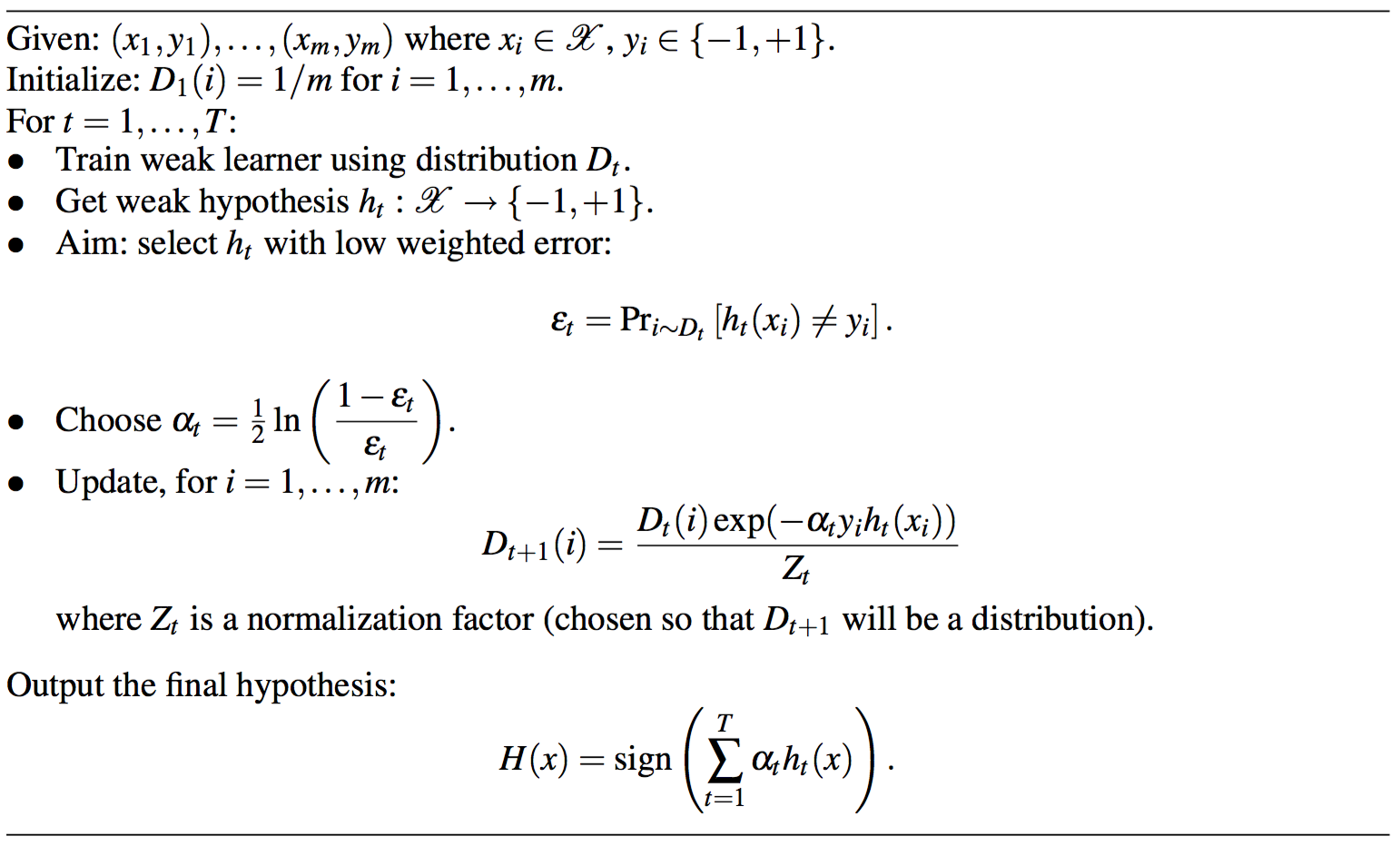
\((x_i, y_i)\) is a tuple where \(x_i\) is features vector and \(y_i\) is class label.
In the begining, all tuples have same weigh represented by distribution \(D_t^i\).
In each iteration, we first train a weak learner using \(D_t\), as long as the learner is better than random guess,
the boosting can get a good result. If the learner is a decision tree, we should consider the weigh when calculating
loss at every tree node for discriminator selection. By using the learner, we can get a weak hypothesis \(h_t\) which maps
features space to {-1, 1}.
\(\epsilon_t\) is the sum of weigh of misclassified tuples. By derivation, \(D_t\) can be updated as above where \(\alpha_t\) equals to
\(\frac{1}{2}ln(\frac{1-\epsilon_t}{\epsilon_t})\).
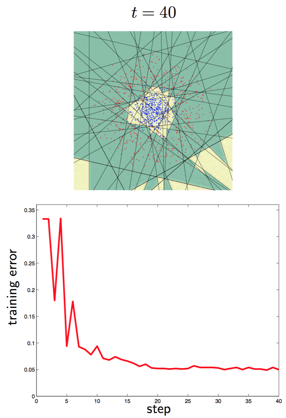
After several rounds, we can get a strong classfier by combining trained weak learner with learner weigh \(\alpha_t\).

Derivation by Loss Function
For simplicity we have \(H(x)=\sum_{t=1}^{T}\alpha_th_t(x)\)
Forward Stagewise Additive Modeling
Input: \(T={(x_1,y_1),(x_2,y_2),…,(x_N,y_N)}\)
Loss Func: \(L(y,f(x))\)
Base Func Set: \(b(x;\gamma)\)
Output: \(f(x)=\sum_{m=1}^{M}\beta_mb(x;\gamma_m)\)
Algorithm:
- Initial\(f_0(x)=0\)
- For m \(\in\) {1,2,3,…,M}
- \((\beta_m,\gamma_m)=arg\min_{\beta,\gamma}\sum_{i=1}^{N}L(y_i,f_{m-1}(x_i)+\beta b(x_i;\gamma))\)
- \(f_m(x)=f_{m-1}(x)+\beta_mb(x;\gamma_m)\)
- \(f(x)=\sum_{m=1}^{M}\beta_mb(x;\gamma_m)\)
We suppose that loss function of Adaboost is exponential loss.
We aim to get
\((\alpha_t,h_t(x))=arg\min_{\alpha,h}\sum_{i=1}^{m}\exp(-y_i(H_{t-1}(x_i)+\alpha h(x_i)))\)
The solution to problem with multiple parameters, we can fix \(H_{t-1}(x_i)\) so that \(\exp(-y_iH_{t-1}(x_i))\) is dependent to
\(\alpha\ and\ h(x_i)\). Set
For solving this equation, \(h_t(x)\) has another equation.
We can solve this by training a weak model.
Consider \(y_i \in \{-1,+1\}\)
From equation above, we can say that \(h_t^{*}(x)\) can replace \(h_t(x_i)\)
Next, we need to get \(\alpha_t\)
\(\alpha_t=arg\min_{\alpha}e^{-\alpha}\sum_{i=1}^{m}D_t^i + (e^{\alpha}-e^{-\alpha})\sum_{i=1}^{m}D_t^iI(y_i \ne h_t^*(x_i))\)
Calculate derivative of the right part and make it 0 to get \(\alpha_t^*\)
We can get
This equation is similar to the update equation in Adaboost except for the normalization coefficient \(Z_t\).
Derivation by Upper Bound
Theorem:
Error is minimized by minimizing \(Z_t\)
Proof:
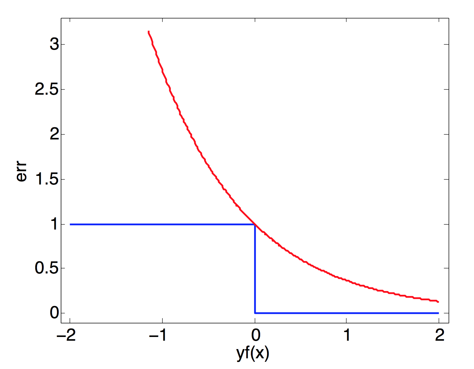
From figure below, we can find that \(I(H(x_i) \ne y_i) \le e^{-y_if(x_i)}\)
 Thus we have
According to this theorem, we should choose \(\alpha_t\) to minimize \(Z_t\)
Remember that \(Z_t\) is the normalization factor, so \(Z_t=\min_{\alpha_t}\sum_{i=1}^{m}D_t^i\exp(-y_i\alpha_th_t(x_i))\)
Making the first derivative of \(Z_t\) with respect to \(\alpha_t\) equals to zero
The result is the same as deviations above.
References
- Improved boosting algorithms using confidence
- AdaBoost Czech Technical University, Prague
- Additive Logistic Regression: a Statistic View of Boosting
- On the Margin Explanation of Boosting Algorithms
- Explaining AdaBoost
- A Decision-Theoretic Generalization of On-Line Learning and an Application to Boosting*